


Using state space methods to estimate Rt

Update: Be sure to check out the update to this post where we gratifyingly produce a huge chart with all the states on it.
Disclaimer: I am not an epidemiologist. Further to what Kevin said, I am not going to try and invent a new model, but rather help estimate an already-existing-one, that was developed by epidemiologists.
The background on this is this post (and this technical notebook) by Kevin Systrom, founder of Instagram, which makes the case that we need to have accurate real-time estimates of Rt, the reproduction number, and provides a methodology for estimating them.
While his approach is clear and awesome, I think that there are two major ways it can be improved:
I could well be wrong about #1, and have misunderstood his procedure at some point. However, the model below, which explicitly models Rt as a moving target, has wider uncertainty near present day viz. Systrom’s model
Systrom’s procedure to estimate
Rtseemed to assume a static Rt, of which we got succesively better estimates with additional data. Ideally we would assume that RtRt could evolve over time (indeed, this seemed to be implictly assumed in the post), but in order to accommodate we need to include some kind of process varianceI had a hard time going through Systrom’s estimation procedure. I am sure it’s right, but it’s also purpose-built for just this problem. If my math is right below, we can use the tried-and-true Kalman Filter to recursively estimate
Rt. This has the advantage of using well-tested approaches; it also brings with it a suite of additional enhancements (like modeling trend, seasonal effects, etc.)
The main equation we start with is (this is equation (2) in the reference paper)
I(t+τ)=I(t)exp(τγ(Rt−1))
Where:
I(t)is the number of infectious people at time t (More on the interpretation of I(t) below)τis the time difference (which for us will always equal one day)γ is the reciprocal of the serial interval (which Systrom sets to 4, so
γ = 1/4)Rt is the number we care about
There is a major issue with I(t). Specifically, we never observe it. All we observe are the number of new cases each day, and the cumulative case count. (And deaths, of course, but this won’t figure in to the analysis below.) As an approximation of the number of infectious people at any point, we can simply use the rolling cumulative sum within the past several days (which I set to 20 in my code)
I am not sure if it boils down to the same issue or not, but Systrom says:
For epidemics that have Rt>1 for a long time and then become under control (Rt<1), the posterior gets stuck. It cannot forget about the many days where Rt>1 so eventually P(Rt|k) asymptotically approaches 1 when we know it’s well under 1. The authors note this in the paper as a footnote. Unfortunately this won’t work for us. The most critical thing to know is when we’ve dipped below the 1.0 threshold!
So, I propose to only incorporate the last m days of the likelihood function.
We have to do something similar. Here’s why:
If we’re modeling:
I(t+1)∼poisson(I(t)exp(γ(Rt−1))
And we use cumulative cases covering the entire history as I(t), then it will always be the case that
I(t+1)≥I(t)
Which implies
exp(γ(Rt−1))≥1
γ(Rt−1)≥0
Rt≥1
So, to allow Rt<1, we need to allow I(t+τ)<I(t), which we can accomplish the same way – by only considering the past 20 days in our analysis.
Using a state space approach seems natural for this problem, since we’re dealing with streaming data that we want to use to recursively estimate a moving target.
Going back to our model setup:
I(t+1)∼poisson(I(t)exp(γ(Rt−1)))
This is exactly equivalent to a poisson regression with an offset or exposure term equal to It.
Pulling from wikipedia, the poisson model is set up as:
E[Y|θ]=exposure∗exp(θ)
We then apply the log link function:
log(E[Y|θ])=log(exposure)+θ
And here, we can substitute γ(Rt−1) for θ and I(t) for exposure. The other change we’ll make is to call γ(Rt−1) = θ
Then a state space model with just an intercept θ(t) and offset = I(t) will be:
I(t+1)∼poisson(I(t)exp(θt))
θ(t)∼N(θ(t−1),σ)
It is this second term in the model that allows us to explicitly model the process variance in the “interest rate” γ(Rt−1)
Doing this in R is straightforward:
First we load our libraries. KFAS is a package for “Exponential Family State Space Models in R”. zoo we use for the function rollsum
library(tidyverse)
library(KFAS)
library(zoo)
#### data ####
url = 'https://raw.githubusercontent.com/nytimes/covid-19-data/master/us-states.csv'
dat = read_csv(url)#### constants ####
WINDOW = 20
SERIAL_INTERVAL = 4
GAMMA = 1 / SERIAL_INTERVAL
STATE = "New York"All we’re doing here is to rebuild the “cumulative cases”, only considering the new cases in WINDOW. We left pad the series to make things line up correctly.
#### building the dataset ####
# rolling window
series =    dat %>%
  filter(state == STATE) %>%
  filter(cases>0) %>%
  pull(cases) %>%
  diff %>%
  {. + 1} %>%
  {c(rep(0, WINDOW-1), .)} %>%
  rollsum(., WINDOW)

# dates dates =
  dat %>%
  filter(state == STATE) %>%
  filter(cases>0) %>%
  pull(date) %>%
  .[c(-1,-2)]
Next, we set up our exposure and dependent variables, which are offsets of each other:
it = series[-length(series)]
itp1 = series[-1]
it here is equal to I(t), and itp1 is I(t+1).
Here, we set up the state space model with a single intercept term:
mod = SSModel(
  itp1 ~ 1,
  u = it,
  distribution = "poisson"
)
u is the exposure parameter. Often you will see this entered into a glm as log(.). However, KFAS in its documentation makes clear that they log this term inside the function
Here, we use KFAS’s way of estimating parameters with maximum likelihood. This corresponds to σσ above (the process variance in θ, which is our “interest rate” γ(Rt−1)
mod$Q[1,1,1] = NA
mod_fit = fitSSM(mod, c(1,1))
Once we’ve estimated σ, we can recursively filter and smooth the θs
mod_fit_filtered = KFS(
  mod_fit$model,
  c("state", "mean"),
  c("state", "mean")
)
We can inspect how the model fits by comparing our one-step-ahead forecasts of cases with actuals (on a log scale):
It’s important to note that these are true forecasts of the day ahead. They are not smoothed values (which would be trivial to extract as well). The reason is that we want to estimate the true uncertainty that a decision-maker would face, which is regarding the estimate of Rt in the future
tibble(
  predictions = mod_fit_filtered$m,
  actuals = series[-1]
) %>%
  mutate_all(~ c(NA, diff(.x))) %>%
  mutate(date = dates) %>%
  .[-1, ] %>%
  gather(-date, key = series, value = value) %>%
  ggplot() +
  aes(x = date, y = value, color = series) +
  geom_line() +
  scale_y_log10("New case count") +
  labs(x = "") +
  scale_color_brewer("", type = "qual", palette = 1) +
  theme(legend.position = c(0.2, 0.8))
Satisfied that the model fits well, we can proceed to estimate where Rt is:
Here we extract the estimates of θ with a traditional 95% confidence interval
theta  = tibble(
  mean_estimate = mod_fit_filtered$a[, 1],
  upper = mean_estimate + 1.96 *
    sqrt(mod_fit_filtered$P[1,1,]),
  lower = mean_estimate - 1.96 *
    sqrt(mod_fit_filtered$P[1,1,])
)[-1, ] # throw away the initial observation
We now have to invert θ=γ(Rt−1)
rt = theta / GAMMA + 1And voilà — we can now plot our estimate of Rt, along with associated uncertainty, over time:
rt %>%
  mutate(date = dates) %>%
  filter(date > lubridate::ymd("20200301")) %>%
  ggplot() +
  aes(x = date, y = mean_estimate,
      ymin = lower, ymax = upper) +
  geom_line(color = "grey") +
  geom_ribbon(alpha = .5, fill = "grey") +
  geom_hline(yintercept = 1) +
  labs(y = "Estimate of Rt", x = "") +
  scale_y_continuous(breaks = c(1,2,3,4)) +
coord_cartesian(ylim=c(NA, 5)) 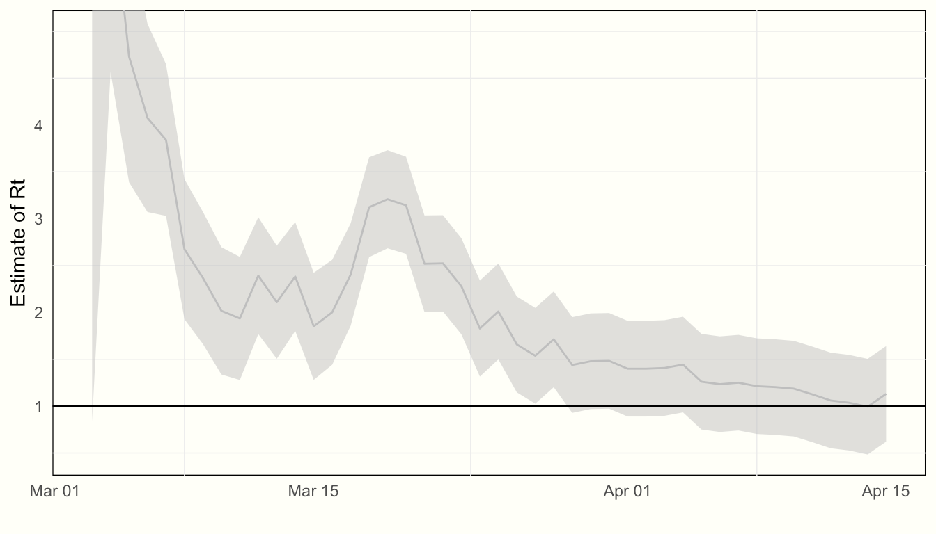
Our final result is 1.13 with standard error 0.26
This is very similar to Systrom’s estimate for New York State:

The main difference, however, is that the uncertainty in the state space version of this model never collapses as far as it does in Systrom’s model. This is due to the fact that we are assuming that γ(Rt−1) (and by extension, RtRt) is a moving target. This is due to the inclusion of θ(t)∼N(θ(t−1),σ) in our model specification
Further extensions of the state space approach could allow for including:
Trend components (both evolving level and slope), and
Seasonal components (e.g. day-of-week, which seems to be present in the data)
Pooling observations across many different time series
Thoughts, questions?
My email is
tom at gradientmetrics dot comThe code for this is here
Some of the most informative work I've read on COVID to date! 👏🏼